Can you write a robot controller directly into its weights?
This experiment applies weight-space programming to a small simulated robot. Fable 5.1 authored the numerical weights of a fixed multilayer perceptron, then revised them using recorded feedback. The useful result is an inspectable reactive controller, with its supporting code and failures available alongside the successful runs.
The primary result is useful reactive motion from directly authored weights, without a conventional mapping or planning stack in the steering loop. The study evaluates that feasibility in simulation; its limits and hardware-transfer questions are stated below.
1. What was tested
The initial objective was to cross the connecting doorway while avoiding the walls. The three-lap mission was a later extension. The model drives in Gazebo Harmonic through two adjoining rooms, approximately 4 × 4 m each, connected by a 0.8 m doorway. Static boxes alter selected passages. ROS 2 Jazzy carries the lidar and velocity commands. The simulated scan has 360 rays, a 6 m maximum range and a nominal 10 Hz update rate.
There are 32 retained episode summaries: 21 door-development runs (003.00–003.20), one three-lap mission (004.01), and ten Nav2 episodes (005.01–005.10). They include weight revisions and scenario changes, not 32 independent trials of one frozen policy. A contaminated earlier 003.00 recording is retained under a discarded filename and excluded from the article's inventory. See RESULTS.md.
2. What “written weights” means
The inspiration is Takehi, Teoh, Zhang and Khattab, *Sparks of Weight-Space Programming*, published 2 November 2026. Their work already includes control and interactive environments. This project explores the idea in a ROS 2 / Gazebo workflow; it does not claim to be the first closed-loop demonstration.
The artifact is policy/write_weights.py: explicit coefficients and biases, organized around geometric predicates. It generates NumPy arrays for a 26 → 16 → 16 → 2 network. Forward evaluation uses tanh at all three layers:
h1 = tanh(W1 x + b1)
h2 = tanh(W2 h1 + b2)
y  = tanh(W3 h2 + b3)
The count is (26×16+16) + (16×16+16) + (16×2+2) = 738 stored coefficients and biases. Most are zero: v01 has 26 nonzero entries, v02 29, v03 73 and v04 78. The constant input x[24] currently has no nonzero outgoing coefficients; explicit bias vectors already provide offsets. This is a sparse, deliberately structured controller embedded in a dense MLP layout, rather than 738 independently discovered decisions.
No gradient descent, reinforcement learning or fitted dataset is used in this implementation. However, failed runs and desk-simulator results informed revisions. This is feedback-guided weight authoring, not a zero-shot evaluation. No language model is called during a navigation episode. Fable 5.1 wrote the weights, analyzed the recorded behavior and activation traces, chose the numerical revisions, and evaluated their effects. Alessandro Pistella supplied the doorway objective and a behavioral suggestion: after observing the robot circling without approaching the door, he told Fable to head toward a wall. He did not supply numerical weights or perform the trace-based diagnosis described below. The source, logs and artifacts document the development; this division of roles reflects Alessandro’s clarification of his contribution.
3. The boundary between network and code
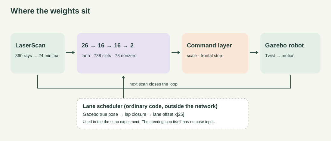
| Component | Responsibility | Information available |
|---|---|---|
| Scan reduction | Minimum range in each of 24 angular sectors, normalized by 6 m | LaserScan |
| MLP | Reactive steering and speed output | 24 reduced ranges, constant x[24], lane offset x[25] |
| Command layer | Scale outputs; stop forward motion below 0.20 m in frontal sectors; publish Twist | Network output and scan |
| Watchdog | Publish zero Twist after missing scans are detected | Wall-clock time since last callback |
| Lane scheduler | Detect a closed lap, advance offset 0 → 0.4 → 0.8, then hold | Pose and traveled distance; true pose in run 004.01 |
| Evaluation / plotting | Outcome, sampled path length and hit-point reconstruction | Gazebo true pose and recorded scans |
The steering network is stateless between scans. The complete mission is stateful, because its scheduler remembers laps and changes an input. True pose influences the next network output through that input. It is therefore accurate to call door following reactive and map-free; it is inaccurate to call the entire three-lap system independent of pose.
The plotted lidar hit map is an offline projection of ranges using true pose, not a SLAM map produced by the network.
4. A worked weight
For the first hidden unit, with d_left measured in metres:
h1[0] = tanh(40 × (d_left − 0.35) / 6)It is near zero at the 0.35 m following distance, positive when the wall is farther away and negative when it is closer. In v04, input x[25] shifts that setpoint:
h1[0] = tanh(40 × (d_left − 0.35 − 1.0 × x[25]) / 6)At offset 0.4, this predicate's target becomes 0.75 m. Other left-facing predicates receive corresponding shifts; the “very close” predicate keeps an absolute threshold. The second layer combines these signals into steering and speed channels; the third reads them out. The names are a design interpretation of explicit equations, not a general technique for reading intentions from arbitrary trained neurons.
The output layer returns values in [−1, 1]. The node computes v = 0.25 × (y[0]+1)/2 and w = 1.0 × y[1]. With every coefficient zero, the robot still moves forward at 0.125 m/s. The empty network is therefore a straight-line reference, not a stationary robot.
5. Why the revisions were made
Doorway priority, v01 → v02. In 003.04 the robot stopped near the jamb. Fable’s analysis of the trace showed that the left-front proximity unit was active, while “wall far” and “left side open” still dominated the left-turn channel. Fable’s v02 revision added a sharper proximity unit (0.34 m threshold, gain 120), subtracted it from that channel and compensated the bias at the following distance. Run 003.05 crossed: the stored episode duration is 23.65 s and sampled path length 5.003 m. The north-wall error on the specified approach segment was 0.0101 m mean. This is wall-following error on a segment, not global localization accuracy.
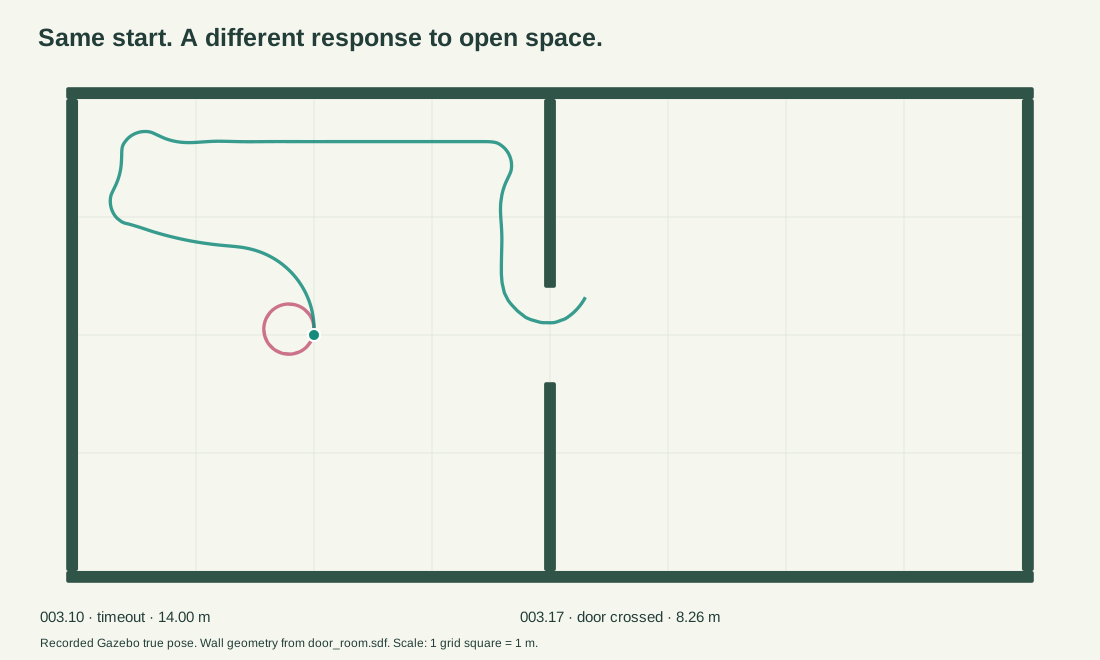
Open-space search, v02 → v03. Run 003.10 started at the room centre and circled until its timeout. The human suggestion was to approach a wall; Fable used the trace and simulation evidence to identify the saturated predicates and work out the corresponding coefficients. With no nearby left wall, the same predicates remained saturated. Fable’s v03 revision suppresses that persistent turning term when the left wall is lost and adds mirrored units comparing left- and right-half scan proximity. The same start crossed in run 003.17: 37.78 s stored episode duration, 8.256 m path. A separate side-aware combination steers toward an open left-front region when an obstacle blocks the front.
Lane offset, v03 → v04. A scalar input changes the wall-distance targets. Code outside the network increments it after detecting lap closure. Run 004.01 completed the three configured laps: 320.64 s stored episode duration and 73.253 m sampled path. The logged lap lengths are 26.26, 24.50 and 19.45 m; they do not sum to the total because acquisition and settling travel are also included.
The final node also differs from an earlier safety implementation: it stops forward motion but allows rotation. That matters for escaping deadlock. The development is therefore not a clean ablation of weights alone. The available files do not prove that every run used byte-identical preprocessing and command logic. A future weight-only comparison must pin the entire node and harness per run.
6. What completion means
Door success in run_door.py is x > 0.3 m and |y| < 0.4 m in Gazebo true pose. It means crossing an evaluation line, not reaching a general requested goal. Stall detection uses small translation and yaw change; a nearest valid scan below 0.10 m then labels the stall “collision.” This is a proxy, not contact-sensor evidence.
For 004.01, the stored label explored means the scheduled laps finished. It does not measure a percentage of observed area, prove complete floor coverage, or identify every reachable frontier. The figure shows a route through both rooms. No quantitative coverage certificate is supplied.
Times quoted in the tables are the JSON field t_end_s, obtained with time.time(). They include harness termination / screenshot overhead after the last sampled pose. For example, 003.15 ends its trajectory at 22.40 s and reports 22.78 s; 004.01 ends its trajectory at 320.08 s and reports 320.64 s. These are wall-clock episode durations, not exact simulation-time crossing latencies. A nominal real-time-factor target of 1 does not verify actual RTF throughout a run.
Paths integrate successive sampled true positions. Policy and Nav2 sampling rates differ, so path lengths have different discretization errors. Summaries, trajectories and the harness definitions are linked in RESULTS.md.
7. Architecture first: a navigation stack and a reactive policy
The primary question is feasibility: can directly authored weights produce useful lidar-driven motion without a conventional mapping / planning stack? Crossing the doorway in seven paired recorded cases is evidence for that narrow claim. The purpose of Nav2 here is to provide an established reference task, not a performance target to beat.
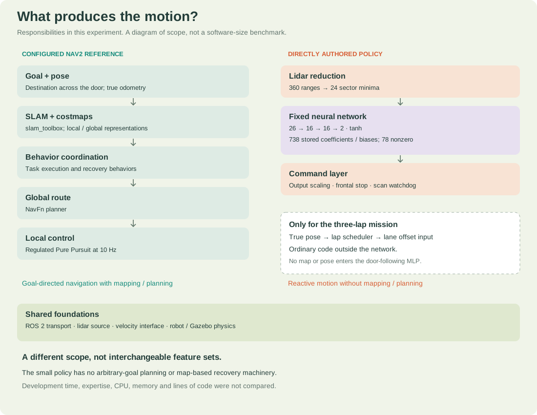
On the configured Nav2 side, SLAM, pose, costmaps, a global planner, a controller and behavior coordination support goal-directed navigation. On the policy side, sector reduction feeds the small MLP and command safeguards. Both still use ROS 2, the scan source and the drive interface. The three-lap policy mission also uses a separate true-pose lane scheduler. The diagram does not equate their feature sets.
A smaller set of navigation responsibilities is visible in this configuration. Lines of code, engineering hours, required expertise, runtime CPU, memory and energy have not been compared. No quantitative savings are claimed for those dimensions.
The comparison uses slam_toolbox, NavFn and Regulated Pure Pursuit, with a fresh SLAM map per door run and true odometry injected by truth_odom_tf.py. The parameter patch sets a 0.12 m radius, 0.25 m/s target speed, 1.0 rad/s limits, a rolling global costmap, 0.30 m inflation radius and a 10 Hz controller. This is a configured baseline, not an untouched default installation.
Both use the same world, paired starts and obstacle specifications. Their tasks and capabilities differ: Nav2 receives a target across the door, while the network follows a wall without receiving that goal. Nav2 can plan on a map and has pose input; it can also reverse, while this policy cannot. Equal nominal limits do not imply identical motion constraints or computational budgets.
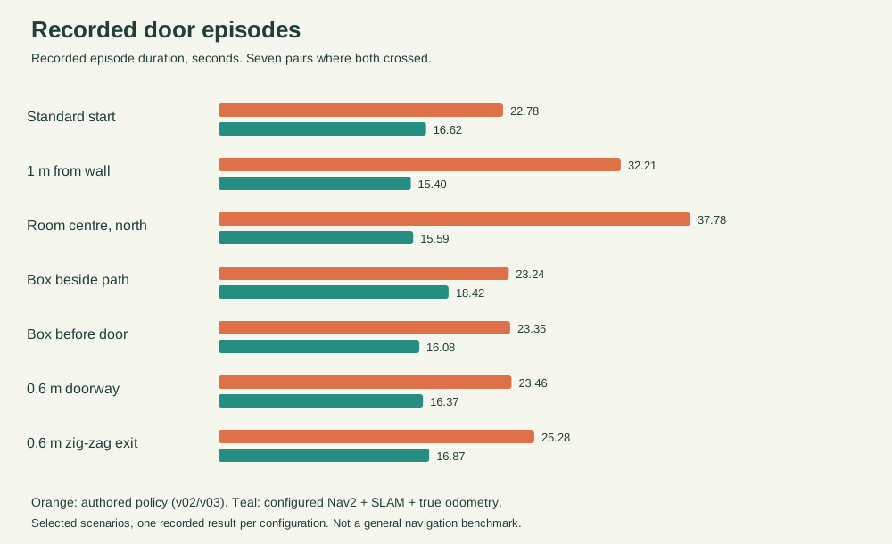
Nav2 is faster in every paired successful door episode. The standard start is 16.62 s / 4.026 m for Nav2 versus 22.78 s / 4.983 m for v03. From the north-facing room centre it is 15.59 s / 2.542 m versus 37.78 s / 8.256 m. The south-facing policy run timed out at 60.64 s; Nav2 crossed in 12.26 s. Neither completed the tested 0.5 m zig-zag case under its own stop / failure criteria. These observations document the different routes; speed and shortest-path optimality were not the feasibility objective. The common failed passage is an interesting shared limit in this setup, not proof of identical failure mechanisms or equivalent general navigation performance.
The exploration runs must not share a speed ranking: explore_lite stops when its frontier criterion is met (005.10, 31.54 s / 4.675 m), whereas 004.01 stops after three laps (320.64 s / 73.253 m). Different termination criteria make a performance ratio meaningless. “No frontiers” is also not a ground-truth coverage proof.
Recorded durations
8. What remains to establish
- A frozen policy on held-out layouts, starts, scan noise and range limitations.
- Repeated trials with process scheduling / physics variation; near-identical runs do not prove universal determinism.
- A coded wall follower with the same preprocessing, scheduler and safety layer.
- Quantitative area coverage and contact-based collision measurement.
- Time-aligned simulation-clock measurements and matched trajectory sampling.
- Real odometry for the mission scheduler, physical scan conventions, footprint and braking-distance checks.
- A real-robot trial. No such result is claimed here.
The outcome worth keeping is modest and concrete: explicit numerical weights can encode a useful small controller, and recorded activations make some failures easy to trace back to a design choice. The repository preserves enough of the experiment to inspect that claim and extend it.
Evidence and reproduction
All retained results · Simulation procedure · Original run log · Command archive · Review findings.